Manual
Press F1 in Signal Visor to open this page.
Your first ten minutes, in this order:
- Open a recording – an IQ file or a Flipper
.sub: Opening a capture. - Look before you decode – the spectrum, the burst, the histogram: The window.
- Read the candidates and the Why column: Analyze.
- When nothing matches, compare frames yourself: Bits.
- Hand the result over to rtl_433, ESPHome or a Flipper: Exports.
You need: nothing but a file. Any receiver that writes
IQ will do, and a Flipper .sub works as well – with the limits in
Flipper RAW. A radio connected to the computer is optional and only
needed for recording.
On this page
How it reads a signal
Everything the program shows comes out of one chain, and it helps to know which step you are looking at when something goes wrong:
samples → envelope → bursts → modulation → pulses → timing → coding → frames → protocol → fieldsBurst detection runs on the envelope whatever the modulation – a frequency-shift transmitter still raises the envelope when it starts and drops it when it stops, so where is there a transmission has the same answer either way. Only the step after it, turning a burst into pulses, depends on how the signal is modulated.
The slicing threshold is not a fixed level. It is derived from the recording itself, because the absolute amplitude depends on the radio's gain, the distance and the antenna, none of which a decoder knows.
Opening a capture
Open reads:
| IQ samples | .cu8, .cs8, .cs16, .cf32, .iq, .complex, .sigmf-data |
|---|---|
| Flipper Zero | .sub RAW – pulse timings only, see below |
An IQ file carries no header, so the sample rate and the format have to come from
somewhere. Signal Visor reads them from the file name when it follows the usual convention
(name_433.92M_250k.cu8); when it cannot, it asks, and tells you what it is missing.
Getting this wrong does not fail loudly – it quietly stretches the spectrum and every timing
measurement with it, so it is worth a second look.
A long recording is never held in memory whole: ten minutes at 2 MSps (2.2 GB) opens in about three seconds and keeps well under a hundred megabytes while it is open. Zooming in to individual pulses reads those few thousand samples back from the file.
Flipper RAW, and why it is a special case
A .sub RAW file contains pulse timings, not amplitude. The envelope
you see for one is reconstructed from those timings and is flagged as such. Two consequences:
- There is no spectrum, no modulation measurement and no signal-to-noise ratio. There is nothing in the file to measure them from.
- Receiver noise was recorded as full-strength pulses, and no threshold can remove it. A noisy
.subtherefore reads as one long burst, and coverage comes out low.
For that second case there is Crop RAW: put cursors A and B around the part you
want, and the program writes a temporary .sub containing only the whole pulses inside
that range. The original file and its preset are left alone.
The window
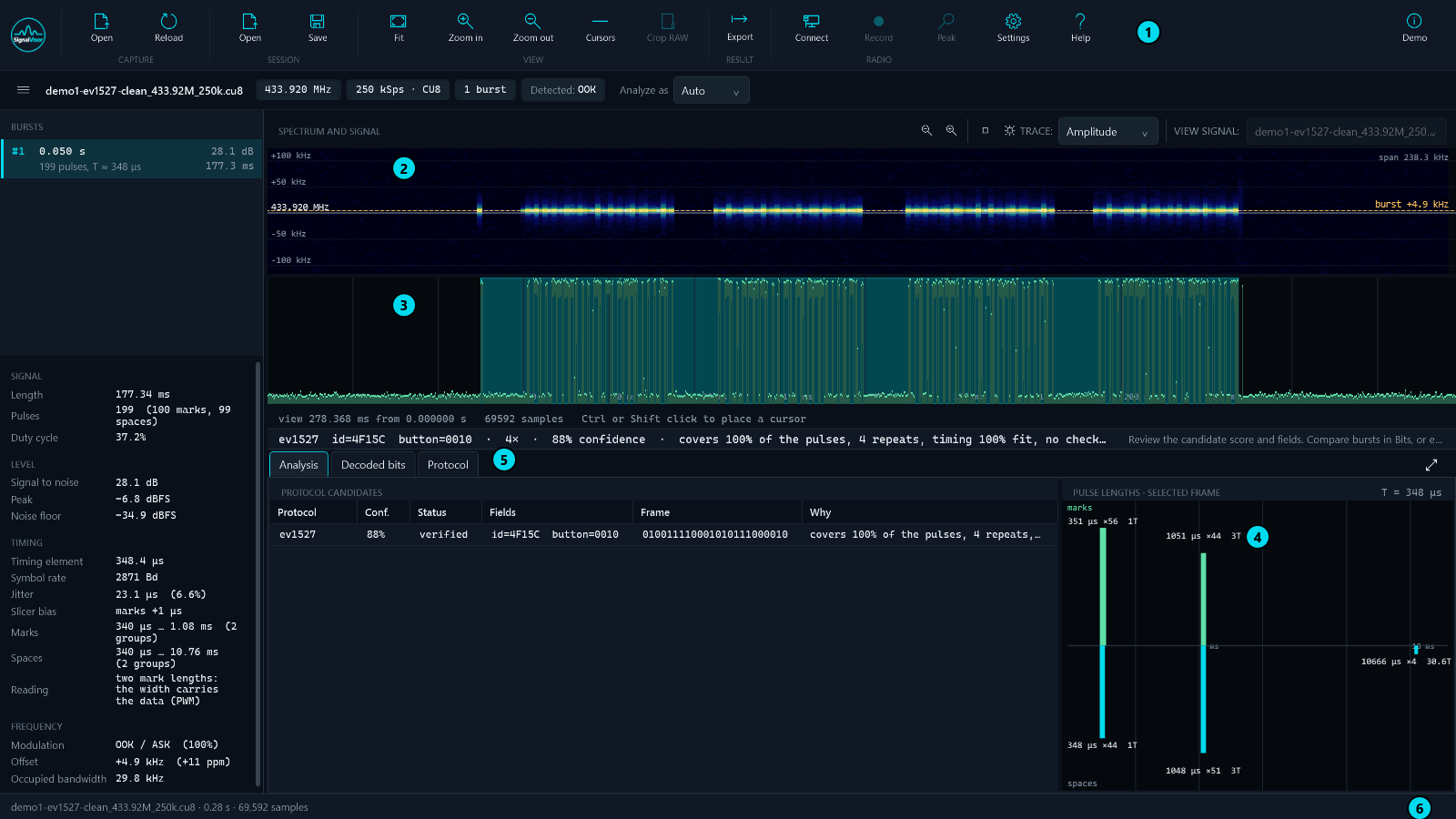
Six areas, top to bottom, numbered as in the picture:
| 1Ribbon | Open, reload, sessions, zoom and cursors, Crop RAW, exports, the radio, then Settings and Help, with Demo on its own at the right edge. One row, because anything you set once and then leave alone belongs in Settings rather than on the toolbar. |
|---|---|
| 2Spectrum | Time across, frequency up, the tuned frequency in the middle. Time runs horizontally on purpose, so the same instant lines up vertically with the timeline below; the two pan and zoom together. A dashed mark shows the burst's measured frequency offset. |
| 3Timeline | The envelope with the detected bursts on it, cursors A and B for direct Δt readout, and a crosshair. Both axes zoom. |
| 4Pulse lengths | The histogram. This is where the structure of a protocol shows up before any decoder runs – see the table below. Clicking a cluster highlights those pulses in the timeline. |
| 5Results | Three workspaces: Analysis (what it is), Decoded bits (what the fields mean) and Protocol (the definitions). Ctrl+1 and Ctrl+2 for the first two. |
| 6Status | The file, its length, the sample count – and the reason when something could not be opened. |
☰ at the left end of the file row hides the burst list and the measurements to give the plots the room, and brings them back at the width they had. The two enlarge buttons above the plots are independent: one gives the whole area to its plot, both give it to the two plots together, and neither restores the usual layout.
Reading the histogram
| What you see | What it means |
|---|---|
| Two mark lengths in a 1 : 3 ratio | PWM – the data is in the pulse width |
| One mark length, two gap lengths | PPM – the data is in the position |
| Everything a multiple of one element | Manchester |
| One gap far longer than the rest | The frame separator |
Analyze
The chip under the ribbon shows the detected modulation. If it is wrong, choose the right one in Analyze as (Auto, OOK, 2-FSK, 4-FSK, BPSK, QPSK, 8-PSK): the whole analysis is redone with it – slicing, statistics, protocol matching and the decoded bits – and the chip then reads “set by hand”. If the capture cannot be measured as that modulation, the automatic result stays and the reason is shown. Trace above the signal plot switches between amplitude and instantaneous frequency; it changes only the view, which makes it a quick check of the detected modulation.
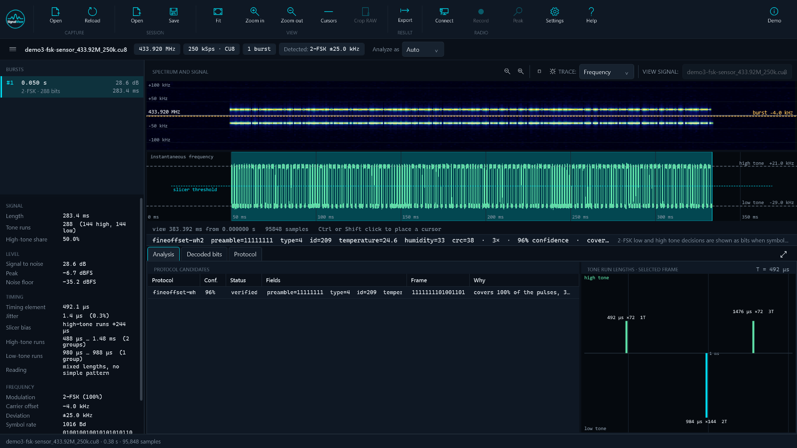
Pick a burst and the table ranks the protocols that fit it. Five columns matter:
- Conf. – how well it fits, mostly pulse coverage and timing agreement.
- Status – verified when a real recording has confirmed the definition, draft when it was written from a datasheet alone. Drafts are ranked lower on purpose: a definition that has never met a signal will often match ones it has nothing to do with.
- Fields and Frame – what it decoded.
- Why – what the confidence is made of. Read this before believing the number above it.
Several protocols matching at once is normal, because many of them are relatives. The measurement panel beside the table gives the burst's timing, jitter, frequency offset and occupied bandwidth, and names the modulation it decided on with the evidence for it.
Sometimes two candidates are the same pulses under two names. The usual pair is EV1527 and PT2262: twelve PT2262 trits are a valid 24-bit EV1527 frame, and both chips set their timing with a resistor, so the timing cannot tell them apart either. The program then shows both with the same confidence, writes “ev1527 or pt2262” in the result line, and says in Why that the signal cannot tell them apart – rather than ranking one first by chance. Only a frame one of them cannot send settles it (a “10” pair rules PT2262 out).
Rolling codes such as KeeLoq (Microchip HCS remotes for gates, garages and alarms) are recognised and split into their visible parts – the encrypted part, the serial number, the buttons – so you know what you are looking at. The encrypted part is shown as received and never decrypted.
Jitter over ten per cent means poor reception or a transmitter that is drifting. A large slicer distortion figure means the threshold is sitting off-centre, and the mark timings should not be taken literally.
Bits
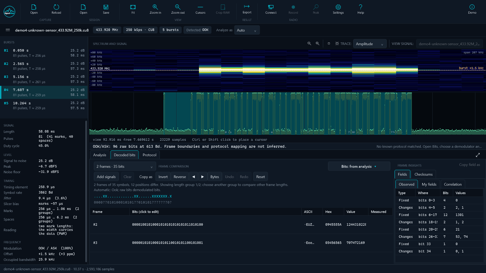
This is the workspace for a device nothing recognises. When no protocol fits, the bits are read from the pulse lengths where the data is in them, as it is for most simple remotes and sensors: two mark lengths (PWM, a long mark is a one) or two gap lengths (PPM, a long gap is a one); frames end at long gaps, and a sync pulse in front of a frame reads as one extra bit to trim. The result line says which reading was used. Anything else is sliced at the recovered symbol rate.
The frames are stacked one above
another, with two rows underneath: the difference mask (a dot where every frame
agrees, an X where they differ) and the common part.
That alone separates the address from the command without decoding anything: what never changes is an identifier, what changes is the button, the state or a counter.
Several recordings at once
Record one button per file and add the files to the comparison – each row carries its source's name and a label you choose („button A, short press“). Press the same button several times first: that is how you tell a stable part of the message from a counter that moves on every transmission. Then compare different buttons.
Frames of different lengths are grouped by length, and you choose which group to compare. Switching groups clears the edits and transforms on purpose – a mask found on a 24-bit frame means nothing on a 40-bit one, and carrying it over silently would produce a plausible-looking answer that is wrong.
The Decode menu
| Bits from | Analysis takes the bits from the analysis (the protocol decoder, when one fits). Raw demodulator takes them straight from the symbol demodulator for the modulation chosen in Analyze as, regardless of protocols; worth it when no frames appear. The modulation itself is chosen only in Analyze as. |
|---|---|
| Line coding | Raw bits, Manchester (either convention), NRZI, UART 8N1/8E1/8N2. |
| Trim frame | Remove bits from either end; the quick version does a bit or a byte. |
| Frame synchronization | Find a repeated word, align every frame on it, and optionally remove it so the payload can be studied on its own. The symbol rate is set here too. |
| XOR whitening mask | A repeating hexadecimal mask over each frame. |
| CC1101 PN9 whitening | Undo PN9 dewhitening with a seed, optionally leaving the preamble and sync bytes untouched. |
Everything here is reversible – Undo, Redo and Reset – and nothing touches the source file. Alignment refuses a pattern that occurs more than once in a frame: it would line every frame up somewhere different and still look consistent.
Fields and checksums
Observed lists what the program found by itself: which positions are constant,
which change, and what values they take. My fields is where you name a range, give
it a format and a scale, and read it as a number across every frame – which is how
0x0D7 becomes 21.5 °C.
The Checksums panel does two things, neither of which changes your data: it compares the usual readings of a frame (normal, inverted, bit-reversed bytes, backwards) to see which one looks like it carries a check, and it searches for a checksum that holds for every compared frame – XOR-8, SUM-8, the common CRC-8 and CRC-16 variants including the CC1101 one, and beyond those it derives an unknown CRC polynomial or LFSR digest from the frames themselves (shown as “derived”). It reports the data range, the position of the check and how strong the evidence is (“5/5 unique payloads”).
Correlation finds a field from real values. Type what you measured for at least three frames into the Measured column – the temperature the display showed, for example – and Find value correlations lists bit ranges, readings and scales that reproduce them. Among equally good fits, round scales (1, 0.5, 0.1…), round offsets and longer ranges come first, because sensors are built that way. Use adds the field to My fields. With few frames and values that move together with a counter, many ranges fit: more frames, more certainty.
The Frame insights panel on the right can be made wider by dragging its left edge.
A match is a candidate, not an identification. Confirm it on frames that were not used to find it – and remember that three buttons sending
0001,0100and1000leave one bit of the button field constant, so the difference mask will call it part of the address. More presses, more certainty.
Protocol
Download JSON definitions and find contribution guidelines in the Signal Visor protocol definitions repository.
The library of every loaded definition on the left – built in or yours, filtered by id, name or classification – and the editor on the right. View / edit JSON… opens the definition as text in its own window, read-only until you switch it to Edit. Below it a checklist says what the definition still lacks, and form tabs (Fields, Coding, Check, Exports, Tests) change one section at a time. The preview shows, as you type, which frames of the selected burst the definition recognises and what it reads from them.
Save writes to your own folder; Export… and Import… move a definition anywhere. Prepare contribution… makes a folder ready to share, with a README that repeats the rules for samples – your own devices only, and no rolling-code captures. Create protocol definition… in Decoded bits starts a draft from what you found there: the frame length, your fields and, when the bits were read from pulse lengths, the coding, the timing element and the symbols as well, so the draft already decodes the recording it came from. A saved definition joins the analysis the next time the program starts.
Demo
Demo, on its own at the right of the ribbon, lists the recordings that ship with the program, each with a line on what to look for, and opens them. They are generated from known values, not recorded from real devices, and are labelled so: that is what lets the program prove its readings against the right answer, and why none of them should be taken for a capture of a real remote or sensor.
Sessions and crash recovery
Save session writes a small .svsession file next to your recording. It
stores the source and its parameters, the selected burst, the workspace, the added comparison
recordings with their labels, your named fields, the decoding settings and the whole
sequence of transforms in the order you applied them.
It stores the recipe, not the result. The frames are recomputed from the recording every time the session opens and the stored sequence is replayed onto them. A session carrying finished bits could disagree with its own source and never say so; a replay either reproduces the same bits or stops and tells you which step no longer fits.
A session written by an older version is converted when you save, and the original is kept beside it
as .bak. The checkpoint for crash recovery is written continuously – after every
transform and every field – so an unexpected exit costs you the view, not the reasoning.
Not stored: cursor positions, zoom, and which candidate row was selected.
Exports
Flipper Zero .sub | Pulse timings the Flipper can replay. |
|---|---|
| rtl_433 flex decoder | A -X decoder line – how a new device reaches
Home Assistant without writing C. |
| ESPHome raw | remote_transmitter.transmit_raw with the measured timings. |
| ESPHome rc_switch | transmit_rc_switch_raw with the protocol described,
which is shorter and editable. |
| RCSwitch protocol | A protocol entry for the Arduino RCSwitch library. |
| Pulse list (CSV) | Every pulse with its length, for a spreadsheet or another tool. |
| Pictures | PNG of the spectrum, the timeline, the histogram, the two together, or the whole window. |
Every exported file carries a header comment naming the capture and this program, so a file found six months later can be traced back to where it came from. Only the exports that make sense for the current result are offered.
Live reception
SDR Connect in the RADIO group connects a receiver; Record writes IQ
to a .cs16 file and Stop opens it for analysis. The dialog remembers what
connected last time – address, frequency, sample rate, filter, gain and the rtl_tcp settings.
Three receivers are supported:
| Receiver | How it connects | Sample rate |
|---|---|---|
| ADALM-Pluto / Pluto+ | LAN tab: its network address. USB tab: its USB network link (192.168.200.22). No driver needed. | 2.083 to 20 MS/s; 2.5 MS/s is a good start |
| HackRF One | USB tab, directly. Needs the WinUSB driver (current firmware installs it by itself). | 2 to 20 MS/s |
| RTL-SDR | USB tab, through rtl_tcp – see below. | up to 2.4 MS/s |
Gain
Use a manual gain. Automatic gain changes the level in the middle of a transmission, and the end of a frame then drops under the slicing threshold. Start around 30 dB with the transmitter a metre or two away; in the measurements panel Peak should sit between about −25 and −10 dBFS and the signal-to-noise ratio above 15 dB. Above −6 dBFS the receiver is overloaded: lower the gain.
- HackRF: the one figure is split the way its documentation advises – the LNA first in 8 dB steps, the rest to the VGA in 2 dB steps (30 dB = LNA 16 + VGA 14; blank = 16 + 16). The front-end amplifier always stays off: with a transmitter on the desk it overloads the receiver and strong signals can damage it.
- RTL-SDR: 0 to 50 dB, rounded by the tuner to its nearest step; blank = automatic.
- Pluto: 0 to about 70 dB; blank = automatic.
RTL-SDR through rtl_tcp
Signal Visor reads an RTL-SDR through rtl_tcp, the small server that comes with the rtl-sdr tools. It is a separate program and not part of Signal Visor. Once set up, the dialog starts and stops it for you. Select the RTL-SDR in the USB tab and the dialog lists the same three steps:
- Driver, once. Run Zadig, choose Options → List All Devices, pick “Bulk-In, Interface (Interface 0)”, set WinUSB and press Replace Driver, then Scan USB again. Until then Windows shows the dongle with an error, and the dialog says the driver is missing.
- rtl_tcp. If you have radioconda, PothosSDR or the rtl-sdr tools in a usual place,
the path is filled in by itself. Otherwise download the Windows x64 release of the
RTL-SDR Blog drivers, unzip it
anywhere and point Browse… at
rtl_tcp.exe. With an empty path, Signal Visor only connects, and you start it yourself:rtl_tcp -a 127.0.0.1 -p 1234. - Connect. If rtl_tcp cannot open the dongle, its own message is shown – a missing driver appears there as a USB error.
The Address field also reaches an RTL-SDR on another computer, where rtl_tcp runs with
-a set to that computer's address. rtl_tcp serves one program at a time: close SDR# or
any other client first.
Lost samples
Every recording is checked two ways, and either result is reported in the status line and the log:
- Against the clock: „~N samples lost in M gap(s)“ when fewer samples arrived than the receiver produced in the time it ran. An estimate, a lower bound: it forgives the receive buffer and a few milliseconds of jitter.
- Against the data: „the receive blocks do not join up“ when the signal jumps at the boundaries between blocks far more than between neighbouring samples – samples went missing between blocks even if the count looks right.
A recording with either warning has gaps written as though no time had passed, so any timing measured across them is wrong. Record again, at a lower sample rate if it repeats. The Pluto also refuses to connect when it does not accept the sample rate asked for, rather than recording at another one.
Files are named after the receiver, frequency, rate and time, e.g.
hackrf_433.92M_2500k_20261114-051200.cs16, and a file that is open for analysis is never
recorded over.
Settings and diagnostics
- Theme – Studio Dark or Blueprint Light. The plots follow: in the light theme the waterfall ramp inverts, so a strong signal prints dark on pale.
- Protocol definitions – two folders. Definitions are available in the
GitHub repository. The built-in one ships with the
program and is read-only; yours is where you put your own
.jsonfiles. A definition with the sameidwins over the built-in one, so a local fix is never overwritten by an update. Settings lists everything that loaded, with its status, and anything that failed to. - Collect diagnostics – packs the rotating local log, the settings in force, the radios the machine can see, the native runtime inventory and the protocol library into one ZIP for a bug report. It works while the program is logging, which is the usual case when something is going wrong.
Nothing is sent anywhere. The log never records the contents of decoded messages, and the archive contains no capture data – see Privacy.
Keyboard
| Timeline | Home whole recording, A / B cursors, Esc clear, ← → pan |
|---|---|
| Spectrum | + − or ↑ ↓ zoom frequency, Home / 0 whole band |
| Histogram | ← → step through clusters, Esc clear the selection |
| Window | Ctrl+1 Analyze, Ctrl+2 Bits, F1 this manual |
Everything in the ribbon is reachable with Tab, and the plots take focus so their keys work without a mouse. Display scaling from 100 % to 200 % is checked by an automated test at six window sizes, not by looking at it.
What it will not do
- It does not transmit. Reception and analysis only.
- It does not help with rolling codes – KeeLoq and the like are recognised and split into their parts, but nothing is decrypted, and opening somebody's car is not what this is for.
- It does not confirm a protocol from a handful of matching frames. Confirmation needs more recordings, or a result known independently – from rtl_433, from a Flipper, from a datasheet with a device in hand.
- It cannot split a noisy Flipper
.subautomatically. Use Crop RAW. - There is no general editable chain of decoding steps yet, and no automatic meaning for a field. The transforms in Bits are individual tools, not a pipeline.
Where something is an estimate, the program says estimate. Where a definition has never been checked against a recording, it says draft. That is deliberate: a confident wrong answer costs more time than no answer.